When one is dealing with statistic or generating random numbers one eventually encounters both the error function and the inverse error function. While some programming languages have the error function included in their math standard libraries, typically the inverse error function is excluded. In this article I will be talking about the inverse error function, some of its uses and go over multiple different methods to approximate it.
The error function (see Figure 1) is the result of integrating a normalized Gaussian function (Normal Distribution).
Unfortunately, there is no closed form expression (evaluates in a finite number of operations) of the inverse error function. Instead the inverse error function is typically defined by an infinite series expansion:
\(erf^{-1}(x)=\sum _{k=0}^{\infty }{\frac {c_{k}}{2k+1}}\left({\frac {\sqrt {\pi }}{2}}x\right)^{2k+1}\)
Where \(c_{0} = 1\) and \(c_{k}\) is:
\(c_{k}=\sum _{m=0}^{k-1}{\frac {c_{m}c_{k-1-m}}{(m+1)(2m+1)}}\)
The first few terms of the inverse error function are:
\(erf^{-1}(x)=\frac{\sqrt {\pi}}{2} \left( x+ \frac{\pi}{12}x^{3} +\frac{7\pi ^{2}}{480}x^{5}+{\frac {127\pi ^{3}}{40320}}x^{7}+{\frac {4369\pi ^{4}}{5806080}}x^{9}+\cdots \right) \)
At first, second and even third glance it is very hard to see the importance of the inverse error function. What makes the inverse error function so important is that it allows you to take a perfectly flat random distribution and transform it into a Gaussian distribution.
As seen in Figure 3, we generated a histogram by generating random numbers between [-1,1] using a flat distribution. We then took each of those random numbers and put it through the inverse error function. Generating a histogram we see that the flat distribution transformed into a Gaussian distribution.
Besides this useful result the inverse error function is used extensively in diffusion calculations and statistics since the inverse error function is the CDF of the normal distribution.
Since we don’t have an equation for the inverse error function that is easily computed we need a way to decide if the accuracy of an approximation function is good enough. What does “good enough” mean?
The answer depends on what type of floating point number you are using. As long as the approximation is more accurate than the floating point number’s precision it can’t be distinguished from the real equation.
The table above lists the highest amount of precision each floating point type is capable of. Therefore for a good approximation all we have to ensure is that the error in the approximation is less than the precision of the floating point number we are using.
The absolute error is the difference between the calculated value \(x_0\) and the real value \(x\):
\(ABS_{Error} = x_0 – x\)
Unfortunatly, as previously stated we don’t have a way to directly calculate the real value of the inverse error function. However, by definition \(erf^{-1}(erf(x))=x\). Since we can calculate \(erf(x)\), the \(ABS_{Error}\) can be calculated as:
\(ABS_{Error}(x) = erf^{-1}(erf(x)) – x\)
Now that we have a way to evaluate approximations we will be looking at four common methods to approximate the inverse error function.
While the inverse error function is defined by an infinite series expansion, the obvious question becomes how many terms does one need to use in order to have a good approximation.
[cpp]
#include <math.h>
double SeriesInverseError10thOrder(const double x){
return 0.8862269254527579 * x + 0.23201366653465444 * pow(x,3) + 0.12755617530559793 * pow(x,5) + 0.08655212924154752 * pow(x,7) + 0.0649596177453854 * pow(x,9);
}
double SeriesInverseError20thOrder(const double x){
return 0.8862269254527579 * x + 0.23201366653465444 * pow(x,3) + 0.12755617530559793 * pow(x,5) + 0.08655212924154752 * pow(x,7) + 0.0649596177453854 * pow(x,9) + 0.051731281984616365 * pow(x,11) + 0.04283672065179733 * pow(x,13) + 0.03646592930853161 * pow(x,15) + 0.03168900502160544 * pow(x,17) + 0.027980632964995214 * pow(x,19);
}
double SeriesInverseError50thOrder(const double x){
return 0.8862269254527579 * x + 0.23201366653465444 * pow(x,3) + 0.12755617530559793 * pow(x,5) + 0.08655212924154752 * pow(x,7) + 0.0649596177453854 * pow(x,9) + 0.051731281984616365 * pow(x,11) + 0.04283672065179733 * pow(x,13) + 0.03646592930853161 * pow(x,15) + 0.03168900502160544 * pow(x,17) + 0.027980632964995214 * pow(x,19) + 0.025022275841198347 * pow(x,21) + 0.02260986331889757 * pow(x,23) + 0.020606780379058987 * pow(x,25) + 0.01891821725077884 * pow(x,27) + 0.017476370562856534 * pow(x,29) + 0.01623150098768524 * pow(x,31) + 0.015146315063247798 * pow(x,33) + 0.014192316002509954 * pow(x,35) + 0.013347364197421288 * pow(x,37) + 0.012594004871332063 * pow(x,39) + 0.011918295936392034 * pow(x,41) + 0.011308970105922531 * pow(x,43) + 0.010756825303317953 * pow(x,45) + 0.010254274081853464 * pow(x,47) + 0.009795005770071162 * pow(x,49);
}
double SeriesInverseError100thOrder(const double x){
return 0.8862269254527579 * x + 0.23201366653465444 * pow(x,3) + 0.12755617530559793 * pow(x,5) + 0.08655212924154752 * pow(x,7) + 0.0649596177453854 * pow(x,9) + 0.051731281984616365 * pow(x,11) + 0.04283672065179733 * pow(x,13) + 0.03646592930853161 * pow(x,15) + 0.03168900502160544 * pow(x,17) + 0.027980632964995214 * pow(x,19) + 0.025022275841198347 * pow(x,21) + 0.02260986331889757 * pow(x,23) + 0.020606780379058987 * pow(x,25) + 0.01891821725077884 * pow(x,27) + 0.017476370562856534 * pow(x,29) + 0.01623150098768524 * pow(x,31) + 0.015146315063247798 * pow(x,33) + 0.014192316002509954 * pow(x,35) + 0.013347364197421288 * pow(x,37) + 0.012594004871332063 * pow(x,39) + 0.011918295936392034 * pow(x,41) + 0.011308970105922531 * pow(x,43) + 0.010756825303317953 * pow(x,45) + 0.010254274081853464 * pow(x,47) + 0.009795005770071162 * pow(x,49) + 0.00937372981918207 * pow(x,51) + 0.008985978502843365 * pow(x,53) + 0.008627953580709422 * pow(x,55) + 0.00829640592773923 * pow(x,57) + 0.007988540162603343 * pow(x,59) + 0.007701938432259749 * pow(x,61) + 0.00743449901783152 * pow(x,63) + 0.007184386511268305 * pow(x,65) + 0.006949991101064708 * pow(x,67) + 0.006729895085341522 * pow(x,69) + 0.006522845161450053 * pow(x,71) + 0.006327729364343136 * pow(x,73) + 0.00614355777038415 * pow(x,75) + 0.00596944626973445 * pow(x,77) + 0.005804602853834295 * pow(x,79) + 0.005648315975551554 * pow(x,81) + 0.0054999446262039555 * pow(x,83) + 0.00535890984168644 * pow(x,85) + 0.005224687403687484 * pow(x,87) + 0.005096801544706202 * pow(x,89) + 0.004974819499739037 * pow(x,91) + 0.004858346774958481 * pow(x,93) + 0.0047470230258849725 * pow(x,95) + 0.004640518455559021 * pow(x,97) + 0.004538530657907072 * pow(x,99);
}
double SeriesInverseError500thOrder(const double x){
return 0.8862269254527579 * x + 0.23201366653465444 * pow(x,3) + 0.12755617530559793 * pow(x,5) + 0.08655212924154752 * pow(x,7) + 0.0649596177453854 * pow(x,9) + 0.051731281984616365 * pow(x,11) + 0.04283672065179733 * pow(x,13) + 0.03646592930853161 * pow(x,15) + 0.03168900502160544 * pow(x,17) + 0.027980632964995214 * pow(x,19) + 0.025022275841198347 * pow(x,21) + 0.02260986331889757 * pow(x,23) + 0.020606780379058987 * pow(x,25) + 0.01891821725077884 * pow(x,27) + 0.017476370562856534 * pow(x,29) + 0.01623150098768524 * pow(x,31) + 0.015146315063247798 * pow(x,33) + 0.014192316002509954 * pow(x,35) + 0.013347364197421288 * pow(x,37) + 0.012594004871332063 * pow(x,39) + 0.011918295936392034 * pow(x,41) + 0.011308970105922531 * pow(x,43) + 0.010756825303317953 * pow(x,45) + 0.010254274081853464 * pow(x,47) + 0.009795005770071162 * pow(x,49) + 0.00937372981918207 * pow(x,51) + 0.008985978502843365 * pow(x,53) + 0.008627953580709422 * pow(x,55) + 0.00829640592773923 * pow(x,57) + 0.007988540162603343 * pow(x,59) + 0.007701938432259749 * pow(x,61) + 0.00743449901783152 * pow(x,63) + 0.007184386511268305 * pow(x,65) + 0.006949991101064708 * pow(x,67) + 0.006729895085341522 * pow(x,69) + 0.006522845161450053 * pow(x,71) + 0.006327729364343136 * pow(x,73) + 0.00614355777038415 * pow(x,75) + 0.00596944626973445 * pow(x,77) + 0.005804602853834295 * pow(x,79) + 0.005648315975551554 * pow(x,81) + 0.0054999446262039555 * pow(x,83) + 0.00535890984168644 * pow(x,85) + 0.005224687403687484 * pow(x,87) + 0.005096801544706202 * pow(x,89) + 0.004974819499739037 * pow(x,91) + 0.004858346774958481 * pow(x,93) + 0.0047470230258849725 * pow(x,95) + 0.004640518455559021 * pow(x,97) + 0.004538530657907072 * pow(x,99) + 0.004440781843527172 * pow(x,101) + 0.004347016395021499 * pow(x,103) + 0.0042569987071827175 * pow(x,105) + 0.00417051127412616 * pow(x,107) + 0.004087352991109011 * pow(x,109) + 0.00400733764349813 * pow(x,111) + 0.003930292559306468 * pow(x,113) + 0.0038560574050482055 * pow(x,115) + 0.003784483107473815 * pow(x,117) + 0.003715430886126037 * pow(x,119) + 0.0036487713836790823 * pow(x,121) + 0.003584383882744558 * pow(x,123) + 0.003522155599297858 * pow(x,125) + 0.0034619810441376495 * pow(x,127) + 0.0034037614448720645 * pow(x,129) + 0.003347404221855558 * pow(x,131) + 0.0032928225123033104 * pow(x,133) + 0.0032399347375042247 * pow(x,135) + 0.0031886642086556213 * pow(x,137) + 0.0031389387673655678 * pow(x,139) + 0.0030906904573240333 * pow(x,141) + 0.00304385522404135 * pow(x,143) + 0.0029983726398996073 * pow(x,145) + 0.002954185652066844 * pow(x,147) + 0.002911240351090823 * pow(x,149) + 0.0028694857582238307 * pow(x,151) + 0.0028288736297367306 * pow(x,153) + 0.0027893582766628493 * pow(x,155) + 0.0027508963985735193 * pow(x,157) + 0.0027134469301298334 * pow(x,159) + 0.002676970899281695 * pow(x,161) + 0.0026414312960976946 * pow(x,163) + 0.0026067929513093027 * pow(x,165) + 0.0025730224237419342 * pow(x,167) + 0.002540087895884912 * pow(x,169) + 0.0025079590769233246 * pow(x,171) + 0.0024766071126183014 * pow(x,173) + 0.0024460045014790908 * pow(x,175) + 0.002416125016721371 * pow(x,177) + 0.0023869436335520523 * pow(x,179) + 0.0023584364613620555 * pow(x,181) + 0.0023305806804456365 * pow(x,183) + 0.0023033544828982926 * pow(x,185) + 0.0022767370173754973 * pow(x,187) + 0.002250708337421751 * pow(x,189) + 0.0022252493531041426 * pow(x,191) + 0.00220034178570695 * pow(x,193) + 0.0021759681252640946 * pow(x,195) + 0.0021521115907245244 * pow(x,197) + 0.002128756092562532 * pow(x,199) + 0.002105886197659956 * pow(x,201) + 0.002083487096301174 * pow(x,203) + 0.0020615445711343583 * pow(x,205) + 0.0020400449679639355 * pow(x,207) + 0.00201897516824968 * pow(x,209) + 0.00199832256319746 * pow(x,211) + 0.001978075029335388 * pow(x,213) + 0.0019582209054771716 * pow(x,215) + 0.0019387489709817671 * pow(x,217) + 0.0019196484252252159 * pow(x,219) + 0.0019009088682066624 * pow(x,221) + 0.0018825202822162794 * pow(x,223) + 0.0018644730144979976 * pow(x,225) + 0.001846757760844751 * pow(x,227) + 0.0018293655500683551 * pow(x,229) + 0.0018122877292901976 * pow(x,231) + 0.0017955159500026674 * pow(x,233) + 0.0017790421548547106 * pow(x,235) + 0.0017628585651180849 * pow(x,237) + 0.0017469576687938258 * pow(x,239) + 0.001731332209321178 * pow(x,241) + 0.0017159751748537467 * pow(x,243) + 0.001700879788069975 * pow(x,245) + 0.001686039496487191 * pow(x,247) + 0.001671447963250492 * pow(x,249) + 0.001657099058369582 * pow(x,251) + 0.001642986850378387 * pow(x,253) + 0.0016291055983939063 * pow(x,255) + 0.001615449744552216 * pow(x,257) + 0.0016020139068009065 * pow(x,259) + 0.0015887928720286174 * pow(x,261) + 0.0015757815895133644 * pow(x,263) + 0.0015629751646726348 * pow(x,265) + 0.0015503688530991604 * pow(x,267) + 0.0015379580548672853 * pow(x,269) + 0.0015257383090957375 * pow(x,271) + 0.0015137052887534616 * pow(x,273) + 0.0015018547956959605 * pow(x,275) + 0.0014901827559203006 * pow(x,277) + 0.001478685215027678 * pow(x,279) + 0.0014673583338830156 * pow(x,281) + 0.0014561983844617347 * pow(x,283) + 0.0014452017458743357 * pow(x,285) + 0.0014343649005600138 * pow(x,287) + 0.001423684430640985 * pow(x,289) + 0.001413157014429672 * pow(x,291) + 0.001402779423081366 * pow(x,293) + 0.0013925485173853214 * pow(x,295) + 0.0013824612446876837 * pow(x,297) + 0.0013725146359399852 * pow(x,299) + 0.0013627058028672803 * pow(x,301) + 0.0013530319352503075 * pow(x,303) + 0.0013434902983163707 * pow(x,305) + 0.0013340782302339149 * pow(x,307) + 0.001324793139706013 * pow(x,309) + 0.0013156325036582665 * pow(x,311) + 0.001306593865016819 * pow(x,313) + 0.001297674830572429 * pow(x,315) + 0.001288873068926738 * pow(x,317) + 0.0012801863085170834 * pow(x,319) + 0.001271612335716371 * pow(x,321) + 0.0012631489930047108 * pow(x,323) + 0.001254794177209685 * pow(x,325) + 0.001246545837812256 * pow(x,327) + 0.0012384019753154882 * pow(x,329) + 0.00123036063967339 * pow(x,331) + 0.0012224199287773018 * pow(x,333) + 0.0012145779869974047 * pow(x,335) + 0.001206833003777016 * pow(x,337) + 0.0011991832122774557 * pow(x,339) + 0.0011916268880714032 * pow(x,341) + 0.0011841623478826993 * pow(x,343) + 0.0011767879483707134 * pow(x,345) + 0.0011695020849574347 * pow(x,347) + 0.001162303190695553 * pow(x,349) + 0.001155189735175876 * pow(x,351) + 0.0011481602234724893 * pow(x,353) + 0.0011412131951241582 * pow(x,355) + 0.0011343472231505362 * pow(x,357) + 0.001127560913101779 * pow(x,359) + 0.0011208529021402775 * pow(x,361) + 0.0011142218581532365 * pow(x,363) + 0.0011076664788949055 * pow(x,365) + 0.0011011854911573118 * pow(x,367) + 0.0010947776499684008 * pow(x,369) + 0.001088441737816534 * pow(x,371) + 0.0010821765639003388 * pow(x,373) + 0.0010759809634029577 * pow(x,375) + 0.0010698537967897648 * pow(x,377) + 0.0010637939491286862 * pow(x,379) + 0.0010578003294322703 * pow(x,381) + 0.001051871870020703 * pow(x,383) + 0.0010460075259049976 * pow(x,385) + 0.0010402062741896442 * pow(x,387) + 0.001034467113493927 * pow(x,389) + 0.0010287890633913458 * pow(x,391) + 0.0010231711638664 * pow(x,393) + 0.0010176124747881504 * pow(x,395) + 0.0010121120753999447 * pow(x,397) + 0.0010066690638247397 * pow(x,399) + 0.001001282556585464 * pow(x,401) + 0.0009959516881398885 * pow(x,403) + 0.000990675610429507 * pow(x,405) + 0.000985453492441922 * pow(x,407) + 0.000980284519786282 * pow(x,409) + 0.0009751678942813104 * pow(x,411) + 0.000970102833555497 * pow(x,413) + 0.000965088570659034 * pow(x,415) + 0.0009601243536870979 * pow(x,417) + 0.0009552094454140942 * pow(x,419) + 0.0009503431229384911 * pow(x,421) + 0.0009455246773378917 * pow(x,423) + 0.0009407534133339981 * pow(x,425) + 0.0009360286489671448 * pow(x,427) + 0.0009313497152800757 * pow(x,429) + 0.0009267159560106687 * pow(x,431) + 0.0009221267272933102 * pow(x,433) + 0.000917581397368642 * pow(x,435) + 0.0009130793463013963 * pow(x,437) + 0.0009086199657060749 * pow(x,439) + 0.0009042026584802059 * pow(x,441) + 0.0008998268385449422 * pow(x,443) + 0.0008954919305927667 * pow(x,445) + 0.0008911973698420738 * pow(x,447) + 0.0008869426017984185 * pow(x,449) + 0.0008827270820222149 * pow(x,451) + 0.0008785502759026872 * pow(x,453) + 0.0008744116584378746 * pow(x,455) + 0.0008703107140205068 * pow(x,457) + 0.0008662469362295634 * pow(x,459) + 0.0008622198276273445 * pow(x,461) + 0.0008582288995618849 * pow(x,463) + 0.0008542736719745464 * pow(x,465) + 0.0008503536732126325 * pow(x,467) + 0.0008464684398468723 * pow(x,469) + 0.0008426175164936275 * pow(x,471) + 0.0008388004556416812 * pow(x,473) + 0.0008350168174834716 * pow(x,475) + 0.0008312661697506358 * pow(x,477) + 0.0008275480875537402 * pow(x,479) + 0.0008238621532260711 * pow(x,481) + 0.0008202079561713666 * pow(x,483) + 0.0008165850927153757 * pow(x,485) + 0.0008129931659611316 * pow(x,487) + 0.0008094317856478317 * pow(x,489) + 0.0008059005680132207 * pow(x,491) + 0.000802399135659376 * pow(x,493) + 0.0007989271174217976 * pow(x,495) + 0.0007954841482417054 * pow(x,497) + 0.0007920698690414611 * pow(x,499);
}
double SeriesInverseError1000thOrder(const double x){
return 0.8862269254527579 * x + 0.23201366653465444 * pow(x,3) + 0.12755617530559793 * pow(x,5) + 0.08655212924154752 * pow(x,7) + 0.0649596177453854 * pow(x,9) + 0.051731281984616365 * pow(x,11) + 0.04283672065179733 * pow(x,13) + 0.03646592930853161 * pow(x,15) + 0.03168900502160544 * pow(x,17) + 0.027980632964995214 * pow(x,19) + 0.025022275841198347 * pow(x,21) + 0.02260986331889757 * pow(x,23) + 0.020606780379058987 * pow(x,25) + 0.01891821725077884 * pow(x,27) + 0.017476370562856534 * pow(x,29) + 0.01623150098768524 * pow(x,31) + 0.015146315063247798 * pow(x,33) + 0.014192316002509954 * pow(x,35) + 0.013347364197421288 * pow(x,37) + 0.012594004871332063 * pow(x,39) + 0.011918295936392034 * pow(x,41) + 0.011308970105922531 * pow(x,43) + 0.010756825303317953 * pow(x,45) + 0.010254274081853464 * pow(x,47) + 0.009795005770071162 * pow(x,49) + 0.00937372981918207 * pow(x,51) + 0.008985978502843365 * pow(x,53) + 0.008627953580709422 * pow(x,55) + 0.00829640592773923 * pow(x,57) + 0.007988540162603343 * pow(x,59) + 0.007701938432259749 * pow(x,61) + 0.00743449901783152 * pow(x,63) + 0.007184386511268305 * pow(x,65) + 0.006949991101064708 * pow(x,67) + 0.006729895085341522 * pow(x,69) + 0.006522845161450053 * pow(x,71) + 0.006327729364343136 * pow(x,73) + 0.00614355777038415 * pow(x,75) + 0.00596944626973445 * pow(x,77) + 0.005804602853834295 * pow(x,79) + 0.005648315975551554 * pow(x,81) + 0.0054999446262039555 * pow(x,83) + 0.00535890984168644 * pow(x,85) + 0.005224687403687484 * pow(x,87) + 0.005096801544706202 * pow(x,89) + 0.004974819499739037 * pow(x,91) + 0.004858346774958481 * pow(x,93) + 0.0047470230258849725 * pow(x,95) + 0.004640518455559021 * pow(x,97) + 0.004538530657907072 * pow(x,99) + 0.004440781843527172 * pow(x,101) + 0.004347016395021499 * pow(x,103) + 0.0042569987071827175 * pow(x,105) + 0.00417051127412616 * pow(x,107) + 0.004087352991109011 * pow(x,109) + 0.00400733764349813 * pow(x,111) + 0.003930292559306468 * pow(x,113) + 0.0038560574050482055 * pow(x,115) + 0.003784483107473815 * pow(x,117) + 0.003715430886126037 * pow(x,119) + 0.0036487713836790823 * pow(x,121) + 0.003584383882744558 * pow(x,123) + 0.003522155599297858 * pow(x,125) + 0.0034619810441376495 * pow(x,127) + 0.0034037614448720645 * pow(x,129) + 0.003347404221855558 * pow(x,131) + 0.0032928225123033104 * pow(x,133) + 0.0032399347375042247 * pow(x,135) + 0.0031886642086556213 * pow(x,137) + 0.0031389387673655678 * pow(x,139) + 0.0030906904573240333 * pow(x,141) + 0.00304385522404135 * pow(x,143) + 0.0029983726398996073 * pow(x,145) + 0.002954185652066844 * pow(x,147) + 0.002911240351090823 * pow(x,149) + 0.0028694857582238307 * pow(x,151) + 0.0028288736297367306 * pow(x,153) + 0.0027893582766628493 * pow(x,155) + 0.0027508963985735193 * pow(x,157) + 0.0027134469301298334 * pow(x,159) + 0.002676970899281695 * pow(x,161) + 0.0026414312960976946 * pow(x,163) + 0.0026067929513093027 * pow(x,165) + 0.0025730224237419342 * pow(x,167) + 0.002540087895884912 * pow(x,169) + 0.0025079590769233246 * pow(x,171) + 0.0024766071126183014 * pow(x,173) + 0.0024460045014790908 * pow(x,175) + 0.002416125016721371 * pow(x,177) + 0.0023869436335520523 * pow(x,179) + 0.0023584364613620555 * pow(x,181) + 0.0023305806804456365 * pow(x,183) + 0.0023033544828982926 * pow(x,185) + 0.0022767370173754973 * pow(x,187) + 0.002250708337421751 * pow(x,189) + 0.0022252493531041426 * pow(x,191) + 0.00220034178570695 * pow(x,193) + 0.0021759681252640946 * pow(x,195) + 0.0021521115907245244 * pow(x,197) + 0.002128756092562532 * pow(x,199) + 0.002105886197659956 * pow(x,201) + 0.002083487096301174 * pow(x,203) + 0.0020615445711343583 * pow(x,205) + 0.0020400449679639355 * pow(x,207) + 0.00201897516824968 * pow(x,209) + 0.00199832256319746 * pow(x,211) + 0.001978075029335388 * pow(x,213) + 0.0019582209054771716 * pow(x,215) + 0.0019387489709817671 * pow(x,217) + 0.0019196484252252159 * pow(x,219) + 0.0019009088682066624 * pow(x,221) + 0.0018825202822162794 * pow(x,223) + 0.0018644730144979976 * pow(x,225) + 0.001846757760844751 * pow(x,227) + 0.0018293655500683551 * pow(x,229) + 0.0018122877292901976 * pow(x,231) + 0.0017955159500026674 * pow(x,233) + 0.0017790421548547106 * pow(x,235) + 0.0017628585651180849 * pow(x,237) + 0.0017469576687938258 * pow(x,239) + 0.001731332209321178 * pow(x,241) + 0.0017159751748537467 * pow(x,243) + 0.001700879788069975 * pow(x,245) + 0.001686039496487191 * pow(x,247) + 0.001671447963250492 * pow(x,249) + 0.001657099058369582 * pow(x,251) + 0.001642986850378387 * pow(x,253) + 0.0016291055983939063 * pow(x,255) + 0.001615449744552216 * pow(x,257) + 0.0016020139068009065 * pow(x,259) + 0.0015887928720286174 * pow(x,261) + 0.0015757815895133644 * pow(x,263) + 0.0015629751646726348 * pow(x,265) + 0.0015503688530991604 * pow(x,267) + 0.0015379580548672853 * pow(x,269) + 0.0015257383090957375 * pow(x,271) + 0.0015137052887534616 * pow(x,273) + 0.0015018547956959605 * pow(x,275) + 0.0014901827559203006 * pow(x,277) + 0.001478685215027678 * pow(x,279) + 0.0014673583338830156 * pow(x,281) + 0.0014561983844617347 * pow(x,283) + 0.0014452017458743357 * pow(x,285) + 0.0014343649005600138 * pow(x,287) + 0.001423684430640985 * pow(x,289) + 0.001413157014429672 * pow(x,291) + 0.001402779423081366 * pow(x,293) + 0.0013925485173853214 * pow(x,295) + 0.0013824612446876837 * pow(x,297) + 0.0013725146359399852 * pow(x,299) + 0.0013627058028672803 * pow(x,301) + 0.0013530319352503075 * pow(x,303) + 0.0013434902983163707 * pow(x,305) + 0.0013340782302339149 * pow(x,307) + 0.001324793139706013 * pow(x,309) + 0.0013156325036582665 * pow(x,311) + 0.001306593865016819 * pow(x,313) + 0.001297674830572429 * pow(x,315) + 0.001288873068926738 * pow(x,317) + 0.0012801863085170834 * pow(x,319) + 0.001271612335716371 * pow(x,321) + 0.0012631489930047108 * pow(x,323) + 0.001254794177209685 * pow(x,325) + 0.001246545837812256 * pow(x,327) + 0.0012384019753154882 * pow(x,329) + 0.00123036063967339 * pow(x,331) + 0.0012224199287773018 * pow(x,333) + 0.0012145779869974047 * pow(x,335) + 0.001206833003777016 * pow(x,337) + 0.0011991832122774557 * pow(x,339) + 0.0011916268880714032 * pow(x,341) + 0.0011841623478826993 * pow(x,343) + 0.0011767879483707134 * pow(x,345) + 0.0011695020849574347 * pow(x,347) + 0.001162303190695553 * pow(x,349) + 0.001155189735175876 * pow(x,351) + 0.0011481602234724893 * pow(x,353) + 0.0011412131951241582 * pow(x,355) + 0.0011343472231505362 * pow(x,357) + 0.001127560913101779 * pow(x,359) + 0.0011208529021402775 * pow(x,361) + 0.0011142218581532365 * pow(x,363) + 0.0011076664788949055 * pow(x,365) + 0.0011011854911573118 * pow(x,367) + 0.0010947776499684008 * pow(x,369) + 0.001088441737816534 * pow(x,371) + 0.0010821765639003388 * pow(x,373) + 0.0010759809634029577 * pow(x,375) + 0.0010698537967897648 * pow(x,377) + 0.0010637939491286862 * pow(x,379) + 0.0010578003294322703 * pow(x,381) + 0.001051871870020703 * pow(x,383) + 0.0010460075259049976 * pow(x,385) + 0.0010402062741896442 * pow(x,387) + 0.001034467113493927 * pow(x,389) + 0.0010287890633913458 * pow(x,391) + 0.0010231711638664 * pow(x,393) + 0.0010176124747881504 * pow(x,395) + 0.0010121120753999447 * pow(x,397) + 0.0010066690638247397 * pow(x,399) + 0.001001282556585464 * pow(x,401) + 0.0009959516881398885 * pow(x,403) + 0.000990675610429507 * pow(x,405) + 0.000985453492441922 * pow(x,407) + 0.000980284519786282 * pow(x,409) + 0.0009751678942813104 * pow(x,411) + 0.000970102833555497 * pow(x,413) + 0.000965088570659034 * pow(x,415) + 0.0009601243536870979 * pow(x,417) + 0.0009552094454140942 * pow(x,419) + 0.0009503431229384911 * pow(x,421) + 0.0009455246773378917 * pow(x,423) + 0.0009407534133339981 * pow(x,425) + 0.0009360286489671448 * pow(x,427) + 0.0009313497152800757 * pow(x,429) + 0.0009267159560106687 * pow(x,431) + 0.0009221267272933102 * pow(x,433) + 0.000917581397368642 * pow(x,435) + 0.0009130793463013963 * pow(x,437) + 0.0009086199657060749 * pow(x,439) + 0.0009042026584802059 * pow(x,441) + 0.0008998268385449422 * pow(x,443) + 0.0008954919305927667 * pow(x,445) + 0.0008911973698420738 * pow(x,447) + 0.0008869426017984185 * pow(x,449) + 0.0008827270820222149 * pow(x,451) + 0.0008785502759026872 * pow(x,453) + 0.0008744116584378746 * pow(x,455) + 0.0008703107140205068 * pow(x,457) + 0.0008662469362295634 * pow(x,459) + 0.0008622198276273445 * pow(x,461) + 0.0008582288995618849 * pow(x,463) + 0.0008542736719745464 * pow(x,465) + 0.0008503536732126325 * pow(x,467) + 0.0008464684398468723 * pow(x,469) + 0.0008426175164936275 * pow(x,471) + 0.0008388004556416812 * pow(x,473) + 0.0008350168174834716 * pow(x,475) + 0.0008312661697506358 * pow(x,477) + 0.0008275480875537402 * pow(x,479) + 0.0008238621532260711 * pow(x,481) + 0.0008202079561713666 * pow(x,483) + 0.0008165850927153757 * pow(x,485) + 0.0008129931659611316 * pow(x,487) + 0.0008094317856478317 * pow(x,489) + 0.0008059005680132207 * pow(x,491) + 0.000802399135659376 * pow(x,493) + 0.0007989271174217976 * pow(x,495) + 0.0007954841482417054 * pow(x,497) + 0.0007920698690414611 * pow(x,499) + 0.0007886839266030129 * pow(x,501) + 0.0007853259734492912 * pow(x,503) + 0.0007819956677284643 * pow(x,505) + 0.0007786926731009741 * pow(x,507) + 0.0007754166586292808 * pow(x,509) + 0.0007721672986702337 * pow(x,511) + 0.0007689442727700021 * pow(x,513) + 0.0007657472655614756 * pow(x,515) + 0.000762575966664118 * pow(x,517) + 0.0007594300705861389 * pow(x,519) + 0.000756309276628966 * pow(x,521) + 0.0007532132887939458 * pow(x,523) + 0.000750141815691205 * pow(x,525) + 0.0007470945704506218 * pow(x,527) + 0.0007440712706348473 * pow(x,529) + 0.0007410716381543222 * pow(x,531) + 0.0007380953991842377 * pow(x,533) + 0.0007351422840833848 * pow(x,535) + 0.0007322120273148497 * pow(x,537) + 0.000729304367368497 * pow(x,539) + 0.0007264190466852019 * pow(x,541) + 0.0007235558115827809 * pow(x,543) + 0.0007207144121835784 * pow(x,545) + 0.000717894602343673 * pow(x,547) + 0.0007150961395836398 * pow(x,549) + 0.0007123187850208579 * pow(x,551) + 0.0007095623033033046 * pow(x,553) + 0.0007068264625448016 * pow(x,555) + 0.0007041110342616792 * pow(x,557) + 0.0007014157933108204 * pow(x,559) + 0.0006987405178290501 * pow(x,561) + 0.0006960849891738388 * pow(x,563) + 0.0006934489918652792 * pow(x,565) + 0.0006908323135293152 * pow(x,567) + 0.0006882347448421842 * pow(x,569) + 0.000685656079476044 * pow(x,571) + 0.0006830961140457571 * pow(x,573) + 0.0006805546480568029 * pow(x,575) + 0.0006780314838542896 * pow(x,577) + 0.0006755264265730298 * pow(x,579) + 0.0006730392840886854 * pow(x,581) + 0.0006705698669699095 * pow(x,583) + 0.000668117988431498 * pow(x,585) + 0.0006656834642885094 * pow(x,587) + 0.0006632661129113348 * pow(x,589) + 0.000660865755181693 * pow(x,591) + 0.0006584822144495324 * pow(x,593) + 0.0006561153164908089 * pow(x,595) + 0.0006537648894661344 * pow(x,597) + 0.0006514307638802585 * pow(x,599) + 0.0006491127725423755 * pow(x,601) + 0.0006468107505272315 * pow(x,603) + 0.0006445245351370161 * pow(x,605) + 0.000642253965864018 * pow(x,607) + 0.0006399988843540261 * pow(x,609) + 0.0006377591343704657 * pow(x,611) + 0.0006355345617592385 * pow(x,613) + 0.0006333250144142678 * pow(x,615) + 0.0006311303422437181 * pow(x,617) + 0.000628950397136883 * pow(x,619) + 0.0006267850329317199 * pow(x,621) + 0.0006246341053830207 * pow(x,623) + 0.0006224974721312038 * pow(x,625) + 0.0006203749926717106 * pow(x,627) + 0.0006182665283249953 * pow(x,629) + 0.0006161719422070947 * pow(x,631) + 0.0006140910992007621 * pow(x,633) + 0.0006120238659271596 * pow(x,635) + 0.0006099701107180854 * pow(x,637) + 0.0006079297035887355 * pow(x,639) + 0.0006059025162109815 * pow(x,641) + 0.0006038884218871508 * pow(x,643) + 0.0006018872955243106 * pow(x,645) + 0.0005998990136090273 * pow(x,647) + 0.0005979234541826043 * pow(x,649) + 0.000595960496816781 * pow(x,651) + 0.0005940100225898867 * pow(x,653) + 0.0005920719140634371 * pow(x,655) + 0.000590146055259164 * pow(x,657) + 0.0005882323316364715 * pow(x,659) + 0.0005863306300703043 * pow(x,661) + 0.000584440838829427 * pow(x,663) + 0.0005825628475550968 * pow(x,665) + 0.0005806965472401283 * pow(x,667) + 0.0005788418302083395 * pow(x,669) + 0.0005769985900943688 * pow(x,671) + 0.0005751667218238599 * pow(x,673) + 0.0005733461215939995 * pow(x,675) + 0.0005715366868544139 * pow(x,677) + 0.0005697383162883983 * pow(x,679) + 0.0005679509097944887 * pow(x,681) + 0.0005661743684683589 * pow(x,683) + 0.0005644085945850407 * pow(x,685) + 0.0005626534915814589 * pow(x,687) + 0.0005609089640392747 * pow(x,689) + 0.0005591749176680341 * pow(x,691) + 0.0005574512592886066 * pow(x,693) + 0.0005557378968169206 * pow(x,695) + 0.0005540347392479788 * pow(x,697) + 0.0005523416966401541 * pow(x,699) + 0.0005506586800997567 * pow(x,701) + 0.0005489856017658699 * pow(x,703) + 0.0005473223747954491 * pow(x,705) + 0.0005456689133486695 * pow(x,707) + 0.0005440251325745404 * pow(x,709) + 0.0005423909485967517 * pow(x,711) + 0.0005407662784997686 * pow(x,713) + 0.0005391510403151626 * pow(x,715) + 0.0005375451530081738 * pow(x,717) + 0.0005359485364645014 * pow(x,719) + 0.0005343611114773172 * pow(x,721) + 0.0005327827997344965 * pow(x,723) + 0.0005312135238060668 * pow(x,725) + 0.0005296532071318631 * pow(x,727) + 0.0005281017740093911 * pow(x,729) + 0.0005265591495818922 * pow(x,731) + 0.0005250252598266081 * pow(x,733) + 0.0005235000315432365 * pow(x,735) + 0.0005219833923425821 * pow(x,737) + 0.0005204752706353906 * pow(x,739) + 0.0005189755956213683 * pow(x,741) + 0.0005174842972783808 * pow(x,743) + 0.0005160013063518285 * pow(x,745) + 0.000514526554344197 * pow(x,747) + 0.0005130599735047725 * pow(x,749) + 0.0005116014968195304 * pow(x,751) + 0.000510151058001182 * pow(x,753) + 0.0005087085914793848 * pow(x,755) + 0.0005072740323911094 * pow(x,757) + 0.0005058473165711607 * pow(x,759) + 0.0005044283805428505 * pow(x,761) + 0.0005030171615088202 * pow(x,763) + 0.000501613597342008 * pow(x,765) + 0.0005002176265767609 * pow(x,767) + 0.0004988291884000804 * pow(x,769) + 0.0004974482226430367 * pow(x,771) + 0.0004960746697722584 * pow(x,773) + 0.0004947084708816159 * pow(x,775) + 0.0004933495676840046 * pow(x,777) + 0.0004919979025032637 * pow(x,779) + 0.0004906534182662187 * pow(x,781) + 0.0004893160584948506 * pow(x,783) + 0.0004879857672985841 * pow(x,785) + 0.0004866624893666964 * pow(x,787) + 0.00048534616996084287 * pow(x,789) + 0.00048403675490769747 * pow(x,791) + 0.00048273419059170677 * pow(x,793) + 0.0004814384239479536 * pow(x,795) + 0.00048014940245513224 * pow(x,797) + 0.00047886707412862724 * pow(x,799) + 0.0004775913875137012 * pow(x,801) + 0.0004763222916787815 * pow(x,803) + 0.0004750597362088536 * pow(x,805) + 0.00047380367119894946 * pow(x,807) + 0.00047255404724773646 * pow(x,809) + 0.00047131081545120245 * pow(x,811) + 0.00047007392739643384 * pow(x,813) + 0.0004688433351554884 * pow(x,815) + 0.0004676189912793587 * pow(x,817) + 0.0004664008487920247 * pow(x,819) + 0.00046518886118459483 * pow(x,821) + 0.00046398298240953506 * pow(x,823) + 0.000462783166874981 * pow(x,825) + 0.0004615893694391351 * pow(x,827) + 0.0004604015454047457 * pow(x,829) + 0.0004592196505136668 * pow(x,831) + 0.00045804364094149806 * pow(x,833) + 0.00045687347329230173 * pow(x,835) + 0.00045570910459339807 * pow(x,837) + 0.00045455049229023415 * pow(x,839) + 0.0004533975942413297 * pow(x,841) + 0.0004522503687132923 * pow(x,843) + 0.00045110877437590826 * pow(x,845) + 0.00044997277029730157 * pow(x,847) + 0.00044884231593916206 * pow(x,849) + 0.00044771737115204495 * pow(x,851) + 0.0004465978961707327 * pow(x,853) + 0.00044548385160966656 * pow(x,855) + 0.00044437519845844244 * pow(x,857) + 0.0004432718980773684 * pow(x,859) + 0.00044217391219308845 * pow(x,861) + 0.0004410812028942648 * pow(x,863) + 0.00043999373262732227 * pow(x,865) + 0.0004389114641922551 * pow(x,867) + 0.00043783436073848575 * pow(x,869) + 0.00043676238576078816 * pow(x,871) + 0.0004356955030952647 * pow(x,873) + 0.0004346336769153805 * pow(x,875) + 0.00043357687172805104 * pow(x,877) + 0.00043252505236978566 * pow(x,879) + 0.00043147818400288325 * pow(x,881) + 0.00043043623211168087 * pow(x,883) + 0.0004293991624988544 * pow(x,885) + 0.00042836694128176836 * pow(x,887) + 0.0004273395348888782 * pow(x,889) + 0.0004263169100561787 * pow(x,891) + 0.0004252990338237038 * pow(x,893) + 0.000424285873532072 * pow(x,895) + 0.00042327739681907923 * pow(x,897) + 0.00042227357161633784 * pow(x,899) + 0.0004212743661459616 * pow(x,901) + 0.0004202797489172942 * pow(x,903) + 0.0004192896887236829 * pow(x,905) + 0.00041830415463929425 * pow(x,907) + 0.0004173231160159738 * pow(x,909) + 0.00041634654248014674 * pow(x,911) + 0.0004153744039297606 * pow(x,913) + 0.0004144066705312683 * pow(x,915) + 0.0004134433127166504 * pow(x,917) + 0.00041248430118047836 * pow(x,919) + 0.0004115296068770157 * pow(x,921) + 0.00041057920101735717 * pow(x,923) + 0.00040963305506660667 * pow(x,925) + 0.00040869114074109053 * pow(x,927) + 0.000407753430005609 * pow(x,929) + 0.0004068198950707221 * pow(x,931) + 0.0004058905083900728 * pow(x,933) + 0.000404965242657743 * pow(x,935) + 0.000404044070805645 * pow(x,937) + 0.0004031269660009469 * pow(x,939) + 0.0004022139016435305 * pow(x,941) + 0.00040130485136348276 * pow(x,943) + 0.0004003997890186193 * pow(x,945) + 0.00039949868869203973 * pow(x,947) + 0.00039860152468971377 * pow(x,949) + 0.0003977082715380997 * pow(x,951) + 0.00039681890398179167 * pow(x,953) + 0.0003959333969811975 * pow(x,955) + 0.0003950517257102469 * pow(x,957) + 0.00039417386555412744 * pow(x,959) + 0.00039329979210705026 * pow(x,961) + 0.0003924294811700424 * pow(x,963) + 0.00039156290874877006 * pow(x,965) + 0.00039070005105138535 * pow(x,967) + 0.00038984088448640336 * pow(x,969) + 0.00038898538566060404 * pow(x,971) + 0.0003881335313769605 * pow(x,973) + 0.00038728529863259393 * pow(x,975) + 0.0003864406646167538 * pow(x,977) + 0.0003855996067088216 * pow(x,979) + 0.0003847621024763423 * pow(x,981) + 0.00038392812967307774 * pow(x,983) + 0.0003830976662370843 * pow(x,985) + 0.00038227069028881605 * pow(x,987) + 0.0003814471801292491 * pow(x,989) + 0.0003806271142380302 * pow(x,991) + 0.00037981047127164726 * pow(x,993) + 0.0003789972300616248 * pow(x,995) + 0.00037818736961273613 * pow(x,997) + 0.00037738086910124255 * pow(x,999);
}
[/cpp]
This approximation relies on a magic number initial approximation but is then refined using Newton’s method. This algorithm is found in many high end mathematic programs such as Matlab. The one drawback of this method is that it requires multiple calls to the error function slowing down the calculation.
Found in Numerical Recipes Third Edition p265, this approximation finds the complimentary inverse error function \(erfc^{-1}(x)\). The complimentary inverse error function can be easily changed to the inverse error function since \(erf^{-1}(x) = erf^{-1}(1-x)\). This approximation uses Halley’s Method in order to find a better approximation to the equation.
Defined in Mike Giles paper, “Approximating the erfinv function”, this approximation is targeted directly at GPUs which rely primarily single (float) point numbers to do their calculations. He sacrificed accuracy in order to dramatically increase the speed at which the function calculates. There is a noticeable deviation in the equation at \(\pm\)0.627271, this is due to jumping to the other equation in the if statement.
Since GPUs calculate in parallel, one of the constraints in the design of this approximation was to make each branch of the if statement take the same amount of time. Due to this constraint the accuracy of the 2nd branch greatly suffered. The 2nd equation doesn’t even have enough accuracy to be used with half precision floating point numbers while the first is accurate for single precision floating point numbers.
If you require absolute accuracy use Newton approximation. To increase it’s speed with a very small hit to accuracy use a single refinement method instead of double refinement. If all you care about is speed and just want an approximation that is somewhat close to the true value, use M. Giles method.

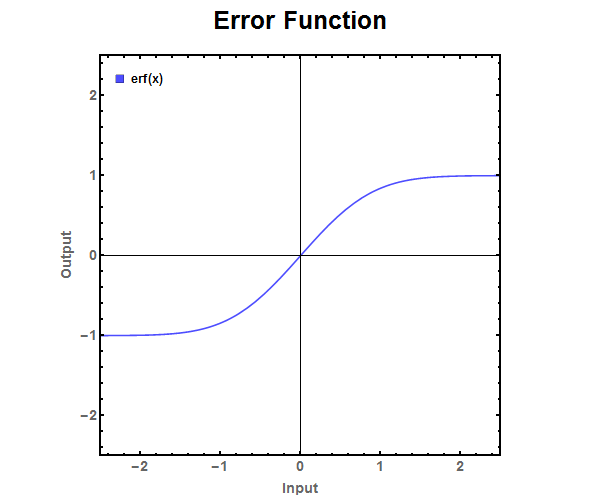 Figure 1: The error function.
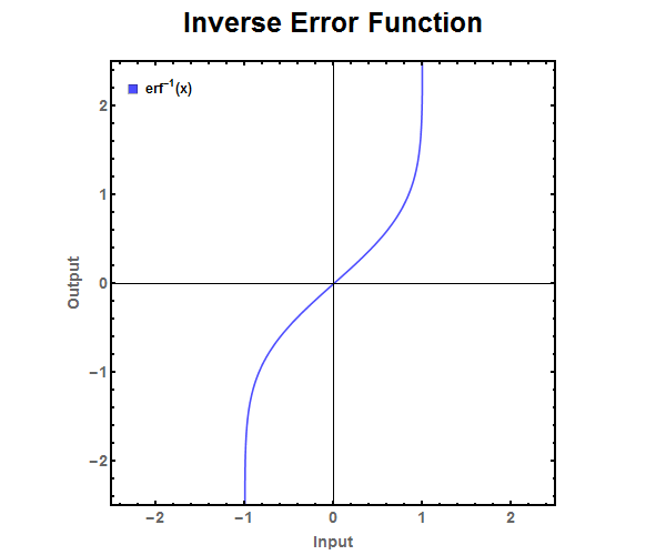 Figure 2: The inverse error function. It ranges from \(-1 \leq x \leq 1 \).
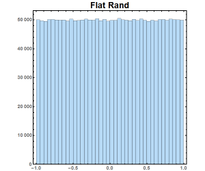
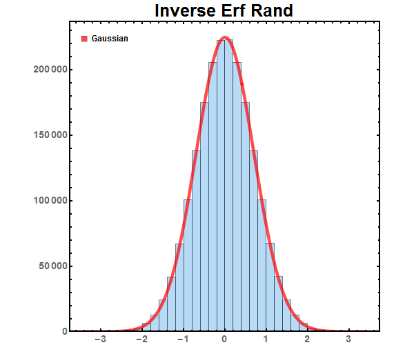
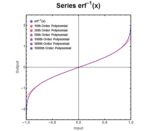 Figure 4: Finite series approximation of the error function.
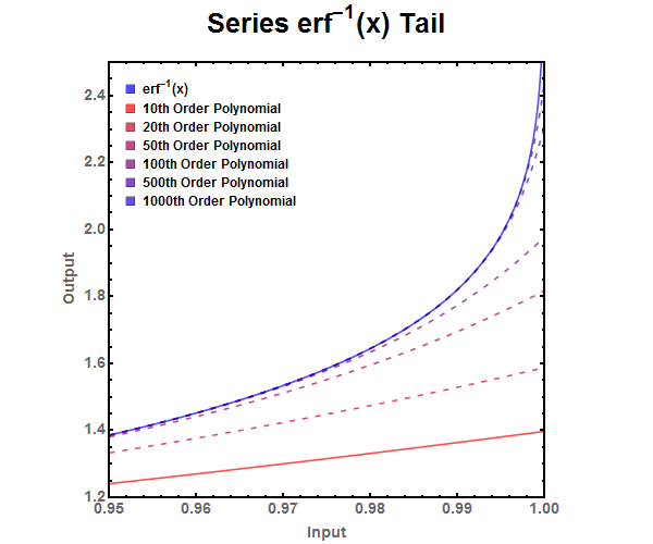 Figure 5: Zoomed look at the tail end of various finite series approximations.
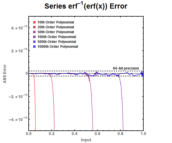 Figure 6: ABS Error for finite series approximation. Notice that the finite series needs to have around 500th order polynomial before it is accurate for double precision floating point numbers.
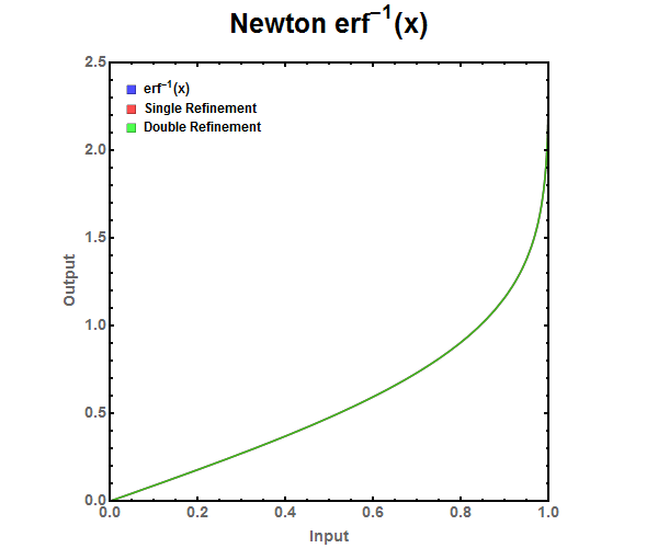 Figure 7: Newton Refinement approximation of the error function. Graphed from 0 to 1 since \(erf^{-1}(-x) = -erf^{-1}(x)\).
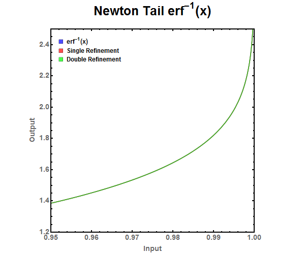 Figure 8: Zoomed look at the tail end of various Newton Refinement approximations. There is no noticeable difference between single and double refinement.
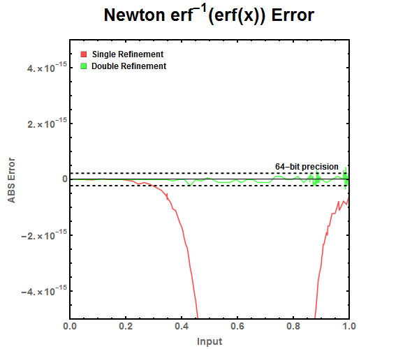 Figure 9: ABS Error for Newton Refinement approximations. Notice that the double refinement is needed to drop the error to the level below double precision floating point numbers while single refinement can be used with single precision floating point numbers.
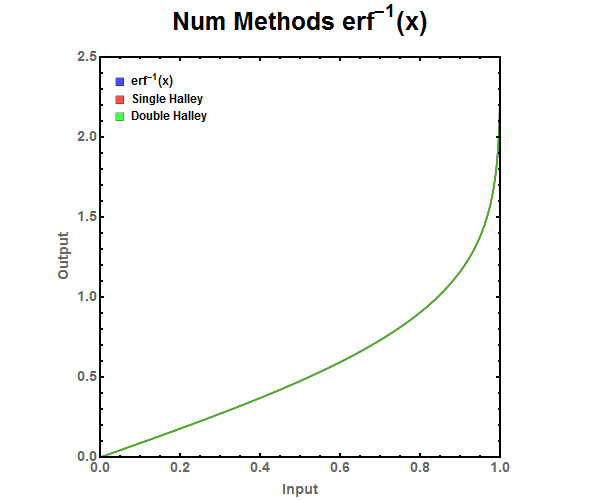 Figure 10: Halley Refinement approximation of the error function.
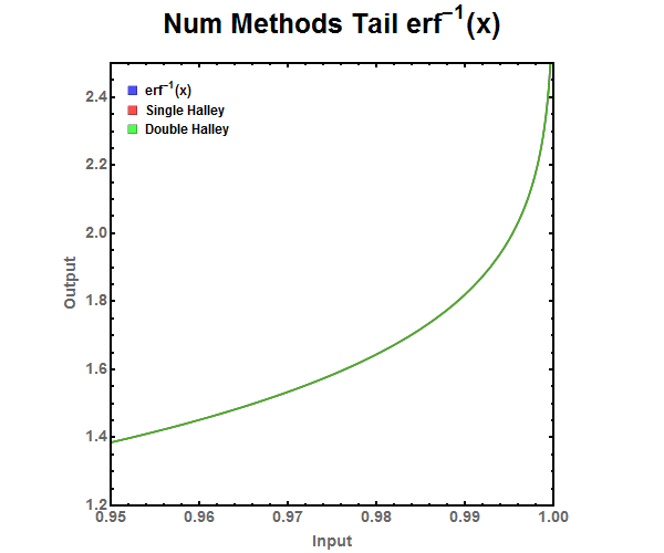 Figure 11: Zoomed look at the tail end of various Halley Refinement approximations. There is no noticeable difference between single and double refinement.
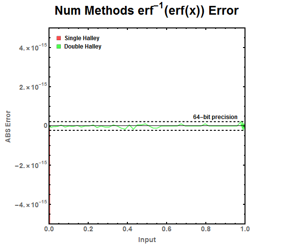 Figure 12: ABS Error for Halley Refinement approximations. Notice that the double refinement is needed to drop the error to the level below double precision floating point numbers while single refinement can be used with single precision floating point numbers.
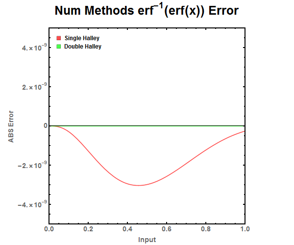 Figure 13: Zoomed out ABS Error for Halley Refinement approximations.
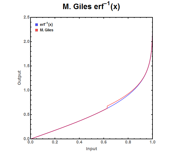 Figure 14: M. Giles approximation of the error function. Jump in the piece wise equation occurs at \(\pm\)0.627271.
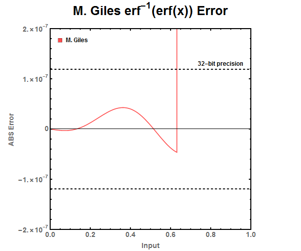 Figure 15: ABS Error for M. Giles approximations. Notice that between -0.627271 \(\leq x \leq\) 0.627271 the error is acceptable for single precision floating point numbers. However outside that range the equation does not have high enough precision for even half precision floating point numbers.
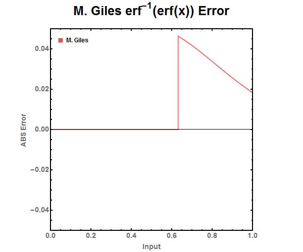 Figure 16: Zoomed out ABS Error for M. Giles approximations.